Utility-based Decisions
UMaine COS 470/570 – Introduction to AI
Spring 2019
Created: 2019-04-25 Thu 21:20
Utility-based reasoning
So far…
- We have explored reflex agents
- We have explored two types of goal-based agents:
- Search agents
- Planning agents
- What about finding the best solution to a goal?
Reflex-based utility agents
- Agent must recognize state \(s\) it is in (or part of it)
- Approaches:
- Agent knows utilities \(U(s)\) and \(U(s')\) of each state \(s'\) reachable from \(s\) by some action \(a\): \[\text{action } = \underset{a}{\arg\!\max}\ U(s'), \text{ s.t. } s\overset{a}{\to}s')\]
- Agent knows quality \(Q(a,s)\) of taking action \(a\) in state \(s\): \[\text{action } = \underset{a}{\arg\!\max}\ Q(a,s)\]
- But: where to get \(U(s)\) or \(Q(a,s)\)?
Utility-based, goal-directed agent
- Concerned with reaching goal in best way
- Local decisions have global consequences
- Could use planner:
- Create all possible plans to achieve goal, pick best
- But planning is NP-hard, so…
- Directly using utilities:
- For each state, determine \(U(s)\) such that overall plan is best
- Or, for each <s,a> pair, determine \(Q(s,a)\) that leads to overall best plan
- But: where to get \(U(s)\) or \(Q(a,s)\)?
Sequential decision problems
Sequential decision problems
- Make sequence of action choices → goal state
- Planning is sequential decision problem
- But here:
- Take (or find) sequence of actions → goal
- Pick the best action in any state with respect to goal
Sequential decision problems
- What information can we use?
- Let \(R(s)\) = reward for state s
- May be able to find \(R\), since it’s local
- Many states may have 0 reward:
\[s_0 \to a_1 \to s_1 \to a_2 \to \cdots a_n \to s_n\]
\[R(s_0)=R(s_1)=\cdots R(s_{n-1})=0\]
- E.g., games, sometimes real world
Markov decision processes
- Formulate SDP as <S,A,T>:
- S = states; distinguished state \(S_0\)
- A = actions; \(A(s)\) = all actions available in s
- T = transition model
- Markov decision process (MDP):
- Fully-observable environment (for now)
- Transitions are Markovian
- Stochastic action outcomes: \(P(s'|s,a)\)
- Rewards additive over sequence of states (environment history)
Policies
- What is solution to an MDP?
- Not just sequence of actions:
- \(S_0\) could be any s
- Stochastic environment could ⇒ not reaching goal state
- Solution is a policy \(\pi\):
- \(\pi(s) =\) action to take in state s
- Agent always knows what to do next
- Policy \(\pi\) ⇒ different environment histories (stochastic env.)
- Expected utility of \(\pi\)
- Optimal policy \(\pi^*\) ⇒ highest expected utility
- \(\pi\) (or \(\pi^*\)):
- is description of simple reflex agent
- computed from info used by utility-based agent
Example world
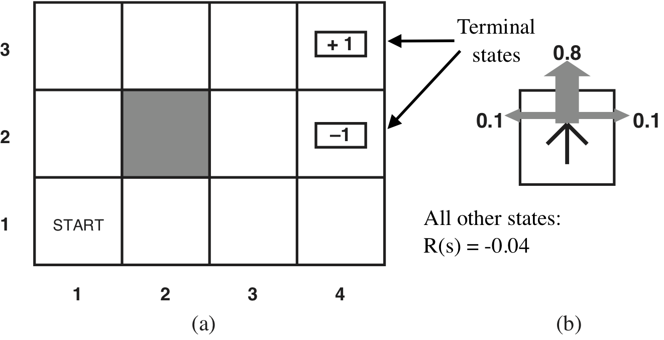
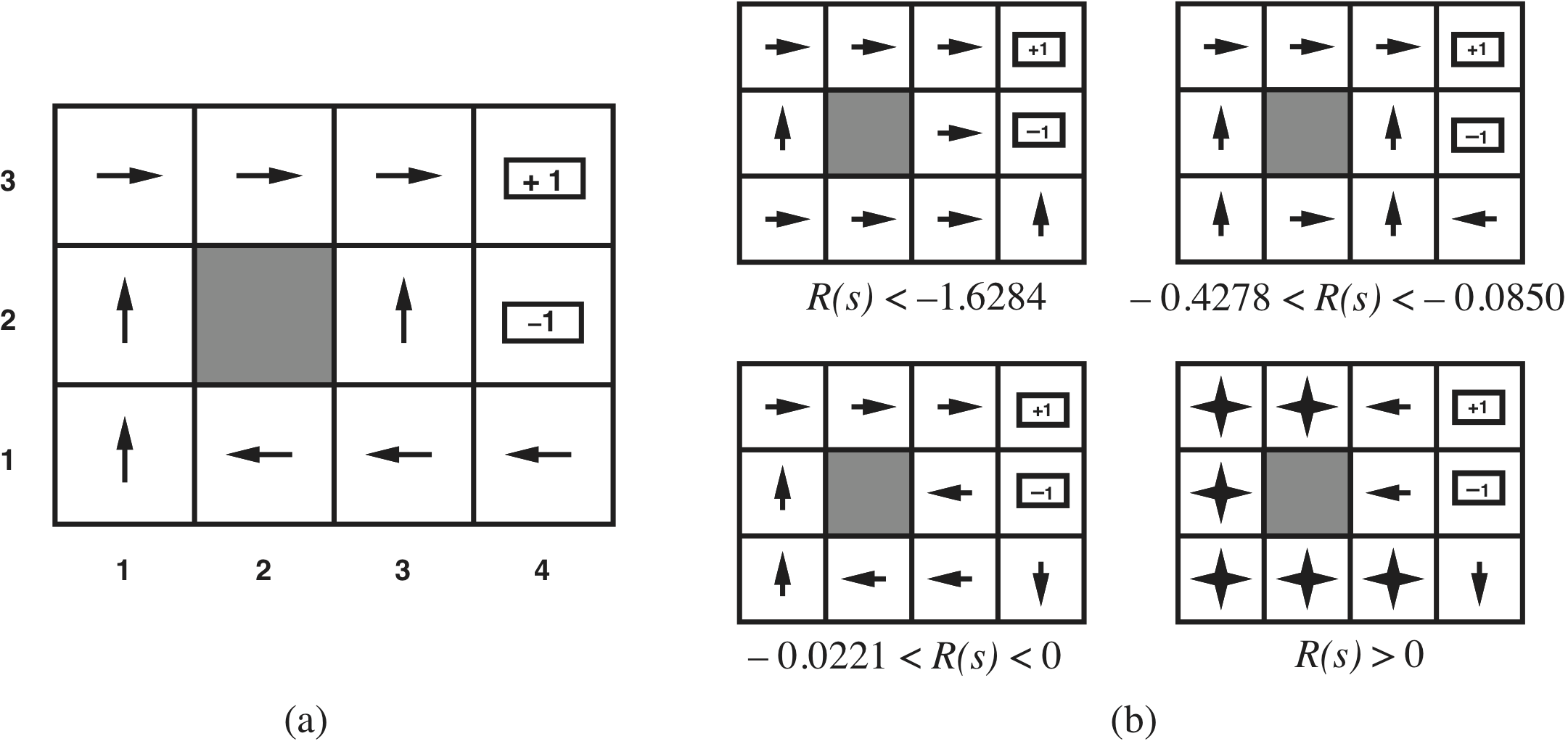
Some optimal policies
Utilities
- Reward \(R(s)\): just depends on \(s\)
- Utility \(U(s)\) of state depends on environment history \(h\) \[U_h([s_0, s_1, s_2, \cdots]) = R(s_0) + \gamma R(s_1) + \gamma R(s_2) + \cdots\] for discount factor \(0\le \gamma \le 1\)
- Discount factor:
- \(\gamma < 1 \Rightarrow\) future rewards not as important as immediate ones
- \(\gamma = 1\): additive rewards
Utilities
- Finite or infinite horizon?
- Finite: game over after some time
- Optimal policy: nonstationary with respect to different horizon
- Short horizon: may choose shorter, but less optimal (or riskier) paths
- Longer horizon: maybe more time to take longer, better paths
- Infinite: game could go on forever
- Optimal policy is stationary
- Optimal action depends only on state
- Simpler to compute
Utilities
- Given a policy, can define utility of a state
\[U^\pi(s) = E[\sum_{t=0}^\infty \gamma^t R(S_t)]\]
where:
- \(S_t\) is state reached at time \(t\)
- Expected value \(\displaystyle E(X) = \sum_{i} x_i P(X=x_i)\)
- Here, expectation is over prob. dist. of state sequences
- \(\pi^* = \underset{\pi}{\arg\!\max} U^\pi(s)\)
- True utility of \(s\) is \(U^\pi(s) = U(s)\)
Optimal policy
- Kind of backward – what we want is \(\pi^*\)
- Can compute \(\pi^*\) if know \(U(s)\) for all states \[\pi^*(s) = \underset{a\in A(s)}{\arg\!\max}\sum_{s'} P(s'|s,a)U(s')\]
- But we said \(U(s) = U^\pi(s)\) – which depends on \(\pi\)!
- How to compute?
Bellman equation
- \(U(s) = R(s) + \) expected discounted utility of next state \[U(s) = R(s) + \gamma \underset{a\in A(s)}{\max}\sum_{s'} P(s'|s,a)U(s')\]
- This is the Bellman equation
- \(n\) states ⇒ \(n\) Bellman equations (one per state)
- Also \(n\) unknowns – utilities for states
- Can we solve via linear algebra?
- Problem: \(\max\) is nonlinear
- So no…
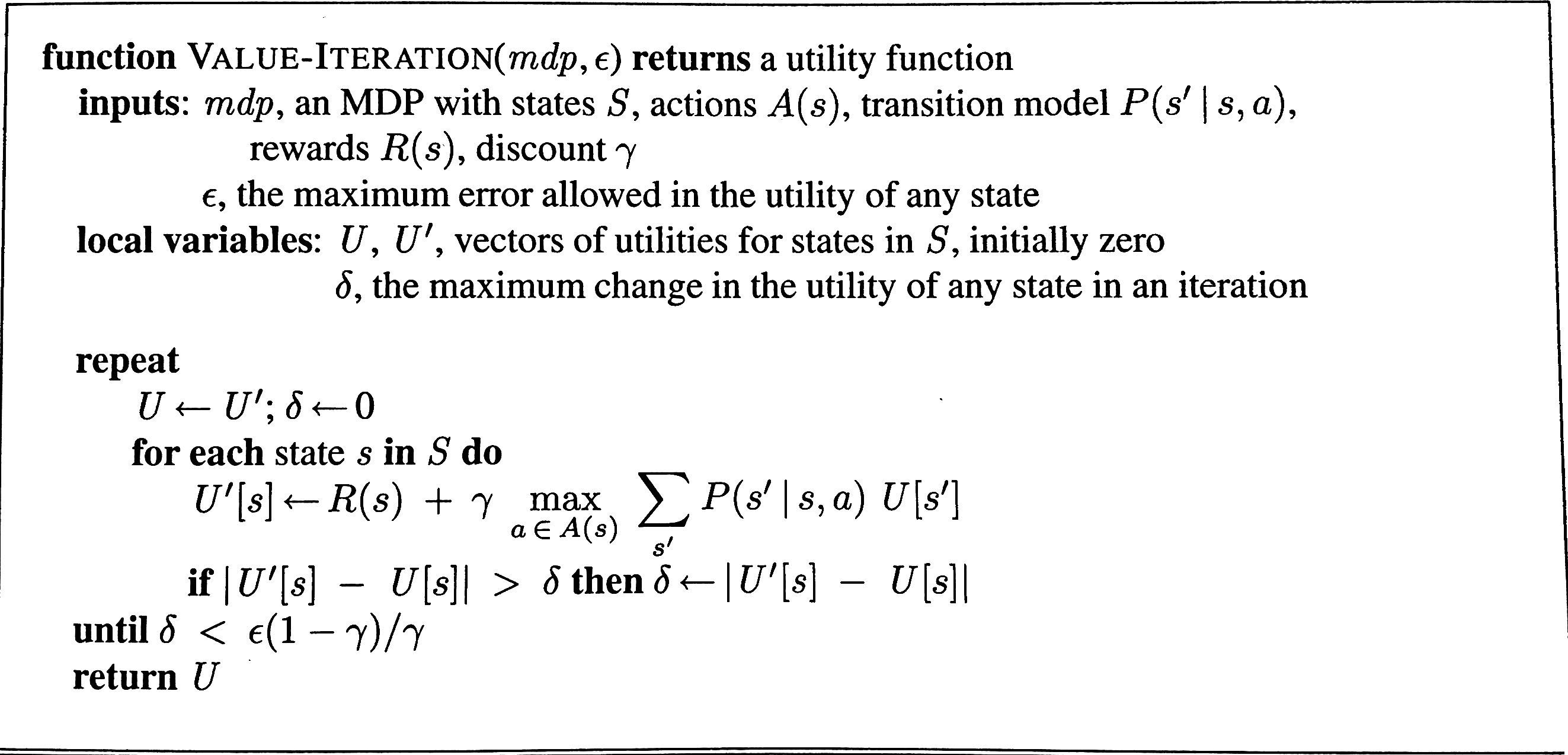
Value iteration algorithm
- Can’t directly solve the Bellman equations
- Instead:
- Start with arbitrary values for \(U(\cdot)\)
- For each \(s\), do a Bellman update: calculate RHS → \(U(s)\)
- Repeat until reach equilibrium (or change < some \(\delta\))
- Bellman update step: \[U_{i+1}(s) \leftarrow R(s) + \gamma \max_{a\in A(s)} \sum_{s'} P(s'|s,a)U_i(s')\]
Algorithm
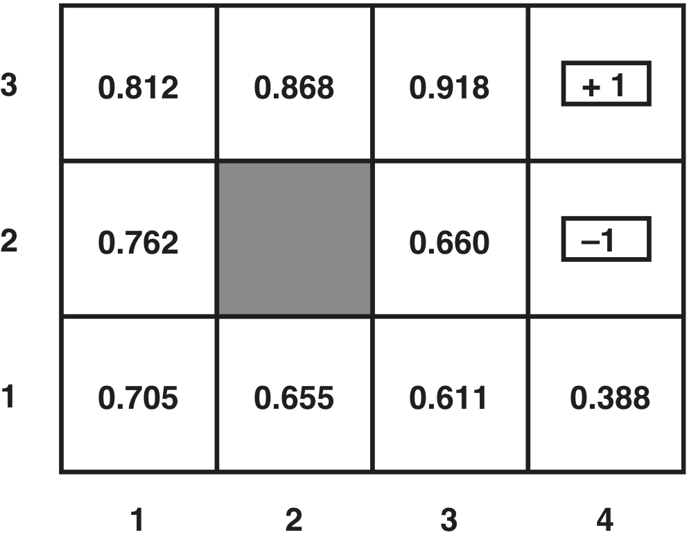
Example
In-class exercise: POP
- No book/notes or online resources
Show how POP would solve this problem (the Sussman anomaly):
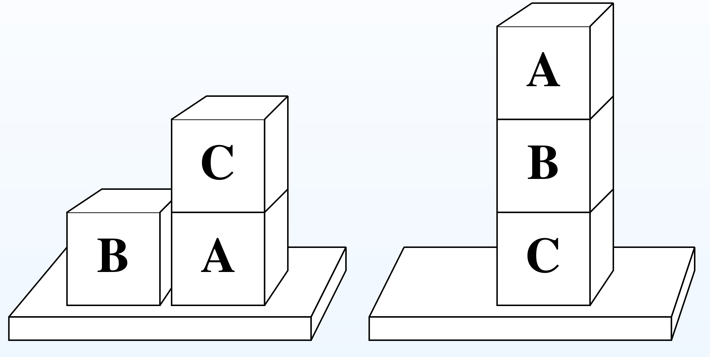
- Initial state: on(B,table), on(A, table), stacked(C,A)
- Goal state: stacked(A,B), stacked(B,C)
- Operators:
- unstack(x,y) – take x off y (and arm will be holding it afteward)
- stack(x,y) – put x (which the arm is holding) on y
- pickup(x) – pick up x from the table
- putdown(x) – put s (which the arm is holding) on the table
In-class exercise: MDPs
Given the example world:
- Use value iteration to find the utilities of the states – stop after 2 iterations
- How do your values compare with those gotten by R&N (above)?
In-class exercise: MDPs
- Draw a transition diagram for the Sussman anomaly
- Use only the actions stack, unstack, putdown, pickup
- Assume that with P(0.1), the arm drops the block when it’s trying to stack it
- Assume with P(0.2), the arm drops the block when it picks it up off the table or off another block
POMDPs
- Assumed environment was fully-observable - but not always the case
- Environment partially-observable ⇒ not sure which state we’re in!
- Sensor uncertainty, sensor incompleteness, incomplete knowledge about interpretation
- Hidden properties of world (“hidden variables”) \[ \text{percept} \Rightarrow s_a | s_b | \cdots\]
- ⇒ Partially-observable Markov decision process (POMDP): much harder
- Real world is a POMDP
POMDPs
- Action in POMDP ⇒ belief state
- Can reason over belief states
- In fact: POMDP ⇒ MDP of belief states
- Can do value iteration to find optimal policy for POMDPs
Summary
- MDP: If we have a model of the environment and reward function, we can learn the optimal policy
- POMDP: Can still do it, using belief state MDP
- But what if we don’t have an environment model or reward function? \[\Rightarrow \textit{ reinforcement learning}\]