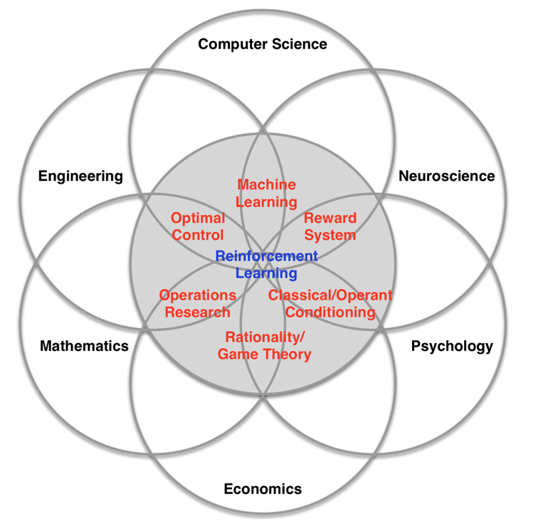
Reinforcement Learning

Why reinforcement learning?

Why reinforcement learning?

• Supervised learning: need labeled examples
• Unsupervised learning: maybe learn structure, but…
• Often:
  • Do not have labeled examples
  • Have to do something – i.e., make some decision – before training is complete
  • But have some feedback about how agent is doing

Framing the problem

• Reinforcement of agent’s actions via rewards
• Current state → choose action → new state + reward
  • Let \(R(s)\) = reward for state s
  • Many states may have 0 reward: \[s_0 \to a_1 \to s_1 \to a_2 \to \cdots a_n \to s_n\] \[R(s_0)=R(s_1)=\cdots R(s_{n-1})=0\]
  • E.g., games
  • Instance of credit assignment problem
• Instance of sequential decision problem

Reinforcement learning

• Rewards
• But no a priori knowledge of rewards, model (transition function)
• E.g.:
  • Given an unfamiliar board and pieces, alternate moves with opponent – only feedback is “you win” or “you lose”
  • Robot has to move around campus delivering mail, but doesn’t know anything about campus, or delivering mail, or people, or…feedback: “good robot”, “ouch!”, falls over, etc.

Reinforcement learning

(From https://icml.cc/2016/tutorials/deep_rl_tutorial.pdf)

Learning approaches

• Learn utilities of states
  • Use to select action to maximize expected outcome utility
  • Needs model of environment, though to know \(s'\) resulting from taking action \(a\) in \(s\)
• Policy learning (reflex agent):
  • Directly learn \(\pi(s)\): which action to take in \(s\), bypassing \(U(s)\)
• Q-learning:
  • Learn an action-utility function Q
  • \(Q(a,s)\) is the value (utility) of action \(a\) in state \(s\)
  • Model-less learning

Learning approaches

• Passive learning:
  • Policy is fixed
  • Task: learn \(U(s)\) (or utility of state-action pairs)
  • Maybe learn model
• Active learning:
  • Has to learn what to do
  • May not even know what its actions do
  • Involves exploration

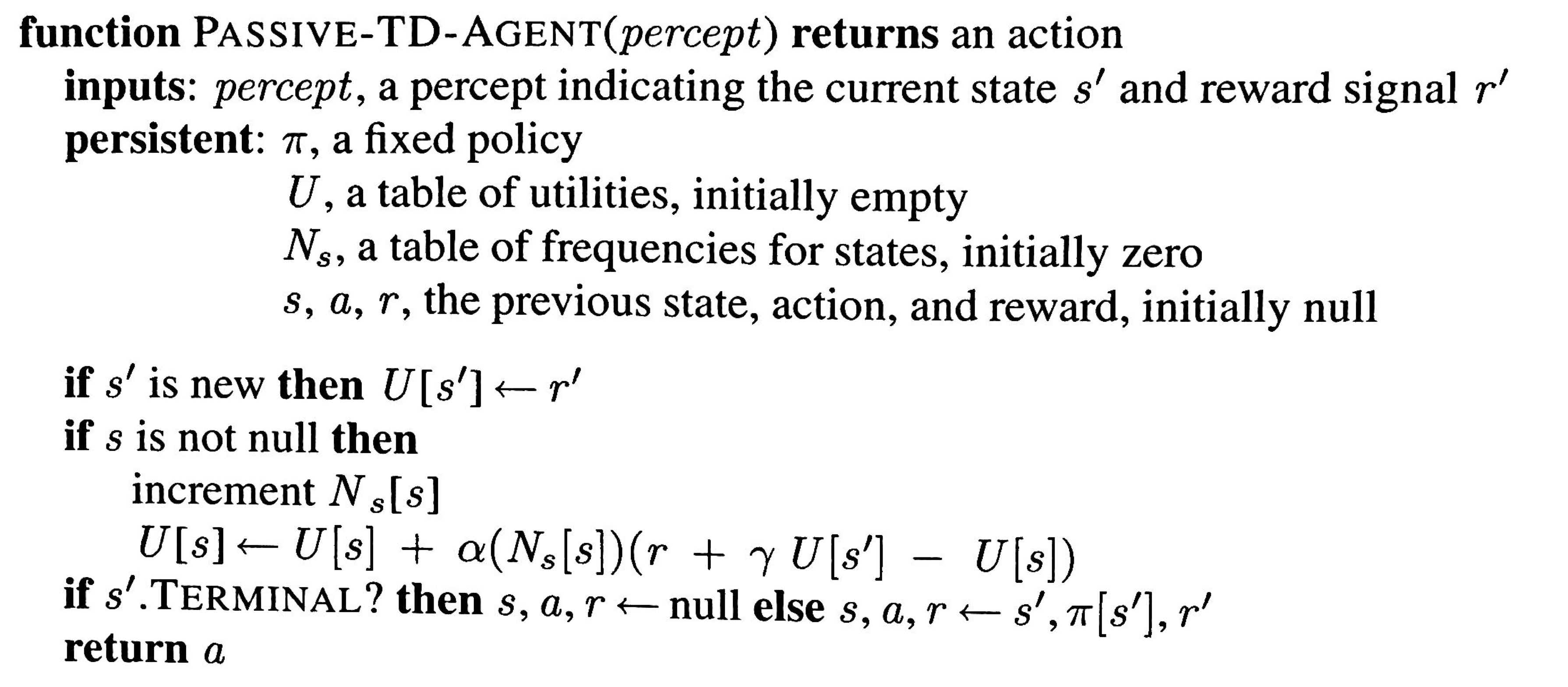
Passive reinforcement learning

Passive reinforcement learning

• Policy \(\pi(s)\) is fixed
• Task: See how good policy is by learning: \[ U^\pi(s) =E\left[ \sum_{t=0}^\infty \gamma^t R(s_t) \right] \]
• Doesn’t know:
  • transition model \(P(s'|s,a)\)
  • reward function \(R(s)\)

• Approach:
  • Do series of trials
  • Each: start at start, follow policy to terminal state
  • Percepts ⇒ new state \(s'\), \(R(s')\)
• Stochastic transitions ⇒ different histories from same \(\pi\)

Direct estimation of \(U^\pi(s)\)

• Woodrow & Huff (1960 – adaptive control theory
• \(U(s)\) = remaining reward = reward-to-go
• View: each trial ⇒ one sample of reward-to-go for each visited state
• Reduces reinforcement learning to supervised learning
• But although \(R(s)\) and \(R(s')\) are independent…
• …\(U(s)\) and \(U(s')\) are not independent – (cf. Bellman equation)
• Misses opportunities for learning – e.g.,
  • See \(s_1\) for first time, it leads to known state \(s_2\) that is known
  • Bellman: \(U(s_2)\) tells us something about \(U(s_1)\)
  • Direct estimation: only \(R(s1)\) matters
• Hypothesis space > needs to be

Adaptive dynamic programming

• First learn model of transition function \(P(s'|s,a)\) from trials
• Now you have an MDP
• Solve it as per sequential decision process
• Could use Bayesian approaches to make this better (see R&N, 21.2.2)

Temporal difference learning

• Use the Bellman equations directly: \[ U^\pi(s) = R(s) + \gamma\sum_s' (P(s'|s, \pi(s))U^\pi(s') \]
• General idea:
  • Start with no known \(U(\cdot)\)
  • Iterate:
    • Take step \(\pi(s)\) to give \(s'\)
    • If \(s'\) is unknown state, use \(R(s')\) as \(U(s')\)
    • Use \(U(s')\) to adjust \(U(s)\) : \[U^\pi(s) \leftarrow U^\pi(s) + \alpha(R(s) + \gamma U^\pi(s') - U^\pi(s))\]

Temporal difference RL algorithm

Active reinforcement learning

Active reinforcement learning

• What if we not only don’t know:

  • \(P(s'|s,a)\)
  • \(R(s)\)

  …also don’t know \(\pi(s)\)?

• One approach: use passive learning, but for all possible actions
  • Use the adaptive dynamic programming agent, but for all \(a\in A(s)\) at each state
  • This gives the transition model
  • Use value iteration or policy iteration ⇒ \(U(s)\)
• Produces greedy agent:
  • Once good terminal state found, tends to keep using policy that found it
  • Seldom in practice converges to optimal policy \(\pi^*\)!

Greedy agent

• Why doesn’t greedy agent converge?
• Only exploits known path – assumes model is good
• But model created based on learned \(\pi\) – leaves some states unexplored
• Actions leading to those states allow better learning of model
• Which allows better estimation of \(U(s)\), \(\pi^*\)
• Have to balance exploitation with exploration

Incorporating exploration

• Using value iteration to get \(U(s)\)
• Now think of \(U^+(s)\), the optimistic estimate of utility of \(s\)
• Design an exploration function \(f(u,n)\) where:
  • \(u\) - expected utility of some new state \(s'\)
  • \(n\) - number of times action \(a\) (expected to lead to \(s'\) from \(s\)) has been tried in \(s\)
• New iteration function for (optimistic) utility: \[U^+(s) \leftarrow R(s) + \gamma \max_a f\left(\sum_{s'} P(s'|s,a)U^+(s'), N(s,a)\right)\] where \(N(s,a) =\) number of times \(s\) has been tried in \(a\)

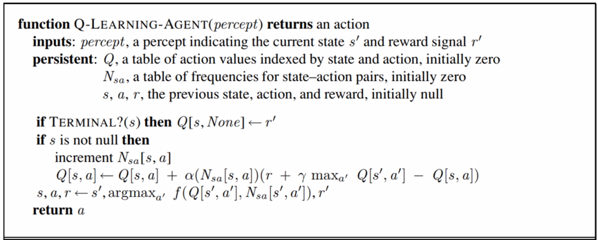
Q-learning

• Instead of learning utilities, learn \(Q(s,a)\): utility of action \(a\) in \(s\)
• Model-free: doesn’t have to know \(U(s)\) at all
• Could do this: \[Q(s,a) = R(s) + \gamma \sum_{s'} P(s'|s,a)\max_{a'}Q(s',a')\]
  • A Bellman equation, but for \(\) pairs rather than \(s\)
  • Could use in adaptive dynamic programming as iteration method
  • But this isn’t really model-free – need \(P(s'|s,a)\)
• Instead, use temporal difference method: \[Q(s,a) \leftarrow Q(s,a) + \alpha(R(s) + \gamma\max_{a'}Q(s', a') - Q(s,a)\]

Q-learning agent

SARSA

• State-action-reward-state-action (SARSA) - similar to Q-learning \[Q(s,a) \leftarrow Q(s,a) + \alpha(R(s) + \gamma Q(s',a') - Q(s,a)\]
• Here, \(a'\) is action actually taken in \(s'\)
• Q-learning: uses best action from \(s'\)
• Still model-free, but have some policy that leads to choosing \(a'\)
• Off-policy vs on-policy algorithms
  • Off-policy algorithms pay no attention to any policy \(\pi\) – e.g., Q-learning
  • On-policy: actions with respect to some policy
• Off-policy more flexible…
• …but if policy is constrained by others (e.g.), may be better to go with realistic actions taken rather than best possible

So…Q-learning or model-learning?

• R&N: “This is an issue at the foundations of artificial intelligence.”
• More generally: do we need models to behave intelligently, or not?
• Traditionally: model (most symbolic AI)
• Lately: model-free (e.g., neural networks)

Generalized RL

Generalized RL

• So far:
  1. Learn \(U(s)\)
  2. Learn \(Q(s,a)\)
• But what if state space is very large or infinite?
• Instead: Learn function approximating \(U(s)\) or \(Q(s,a)\) – \(\widehat{U}(s)\) or \(\widehat{Q}(s,a)\)
• E.g., approximate \(U(s)\) by linear combination of features
  • Static eval for chess, etc.
  • \(\widehat{U}(s) = \theta_1 f_1(s) + \cdots \theta_n f_n(s)\)
  • Just learn \(\theta_i\) values
  • For chess, \(> 10^{40}\) states – now only learn \(n\) values, where \(n <\!< 10^{40}\)
• Not just save space: allows generalization
• On the other hand: maybe we choose wrong hypothesis space

Generalized RL

• So – how to approach?
• One way:
  • Choose utility approximator
  • Run a series of trials
  • Find best fit of feature weights to data (min. squared error)
  • ⇒ Supervised learning

Generalized RL

• Better to use online algorithm for RL
  • Estimate \(\widehat{U}(s)\) (random to start)
  • Run trial
  • Adjust $\widehat{U(s)} accordingly
• How to adjust?
  • Compute gradient with respect to each parameter
  • Move parameter down gradient
  • Sound familiar?

Generalized RL: Delta rule

• Widrow-Hoff rule (delta rule)
• For trial \(j\), observed utility \(u_j(s)\), and parameters \(\theta\), let error: \begin{eqnarray*} E_j(s) &=& (\widehat{U}_θ(s) - u_j(s))²/2
  ∇ E_θi &= & ∂ E_j/∂θ_i
  θ_i &←& θ_i - α\frac{\partial E_j(s)}{\partial \theta_i}
  &←& θ_i + α(u_j(s) - \widehat{U}_θ(s) ) \frac{∂ \widehat{U}_θ(s)}{∂ θ_i}
  
• The \(\theta\) parameters can also be the weights in a neural network!

Deep reinforcement learning

Deep reinforcement learning

• In RL, we can learn:
  • \(U(s)\)
  • \(Q(s,a)\)
  • \(\pi(s)\)
• In generalized RL: learn parameters \(\theta\) of functions approximating \(U\), \(Q\), \(\pi\)
• Inputs: percepts
• Outputs: actions
• Have to know form of function (hypothesis space)
• Deep learning: excels in learning nonlinear functions mapping inputs to outputs
• Maybe combine RL and DL ⇒ deep reinforcement learning

Model learning

• Need to learn \(U(s)\), \(P(s'|s,a)\)
• Either/both can be learned by DL
• DL is responsible for understanding what the state s is given percepts
• E.g., for \(U(s)\):
  • Weights \(\theta\)
  • Many trials
  • Each trial: \[\theta\leftarrow \arg\!\min_\theta \frac{1}{2} \sum_i ||U_\theta^\pi(s_i) - y_i ||^2\]
  • Compute \(y\) the target value via Monte Carlo method
    • Using policy, go from \(s\) to end to find utility
    • Average multiple trials
• Or use Bellman equation, with temporal difference
  • Now, however: don’t store \(U(s)\) – adjust the NN’s weights

Deep Q-learning

• Can we use deep learning to do model-free Q-learning?
• Deep Q-network (DQN):
  • Function approximating \(Q(s,a)\): \(Q(s,a;\theta)\)
  • Here, \(\theta\) are the parameters: the weights of NN
• Problem: Can’t just treat as supervised learning problem
  • Q-learning isn’t stable w/ DL
  • Q-learning balances exploitation with exploration
  • ⇒ Input space, actions – changing as we explore more
  • As these change, target value for \(Q\) changes
  • So net’s input space, output space changing rapidly as explore

DQN

• Train by minimizing sequence of loss functions: \[L_i(\theta_i) = E\left[(y_i-Q(s,a; \theta_i))^2 \right]\] where \(y_i\) is the target: \[y_i = E\left[r+\gamma\max_{a'} Q(s',a'; \theta_{i-1})|s,a\right]\]
• \(s\) here is a sequence of states here (so not Markovian?)
• Expected value for \(L\) based on probability function over sequences of states
• Target determined from emulator/world + previous \(\theta\)
• Optimize loss function \(L_i(\theta_i)\) with parameters from previous iteration \(\theta_{i-1}\) held fixed
• Target depends on weights – not like supervised learning
• Gradient \[\nabla_{\theta_i} L_i(\theta_i) = E\left[(r+\gamma Q(s',a';\theta_{i-1}) - Q(s,a; \theta_i)\nabla_{\theta_i} Q(s,a;\theta_i)\right]\]
• Use stochastic gradient descent

DQN

• As implemented by Mnih et al. (2013) at DeepMind
• Use past experience, past weights to slow down changes in input, output space
• Allows gradual learning of \(Q\)
• Experience replay:
  • Keep last million or so <\(s,a,r\)> in replay buffer
  • Train using batches from here
• Target network:
  • Use two networks
  • Update one constantly
  • Other (target net): synchronize with other occasionally
  • Target network provides \(Q\) values instead of using the rapidly-changing one
  • So: \(Q\) from old weights trains new weights, then new becomes old occasionally

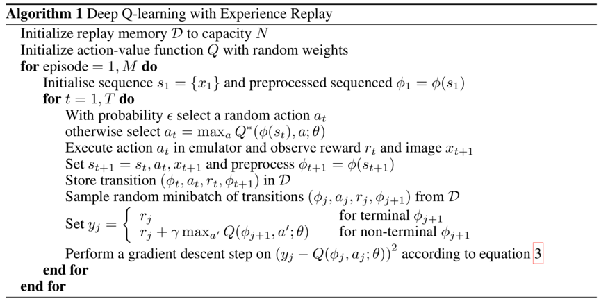
DQN algorithm

DQN results

• DeepMind’s early work:Atari games
• Played most better than any other RL program, some better than humans
• Input: raw frames (201 × 160 pixels, 128 colors)
• Output: actions
• Pre-processing: convert to grayscale, downsample + crop to rough game area
• Convolutional neural network
  • First layer: 16 8 × 8 filters, stride 4, ReLu
  • Second layer: 32 4 × 4 filters, stride 2, ReLu
  • Last hidden layer: fully-connected, 256 ReLu units
  • Output: Fully connected linear layer, single output per valid action

Example: ConvNetJS

Double DQN

• Q-learning problem: can be overly optimistic on value of \(Q\) due to approximation error
• Update function for Q-learning \[\theta_{t+1} = \theta_t + \alpha(Y_t - Q(s_t, a_t; \theta_t))\nabla_{\theta_t} Q(s_t, a_t; \theta_t)\] where: \[Y_t \equiv R(s_{t+1}) + \gamma \max_a Q(s_{t+1}, a; \theta_t)\]
• For DQN: \[Y_t \equiv R(s_{t+1}) + \gamma\max_a Q(s_{t+1},a,\theta^{-}_t)\]
• \(\max_a\) portion: target weights select and evaluate best action it would take
• May not be action that online net selects ⇒ possible overestimate

Double DQN

• Best if “best action” is one online net would choose…
• …but estimated target is per target net
• ⇒ Double DQN target: \[Y_t \equiv R(s_{t+1} + \gamma Q(s_{t+1}, \arg\!\max_a Q(s_{t+1},a; \theta_t); \theta^{-}_t)\]
• Much better learning due to fewer overestimates

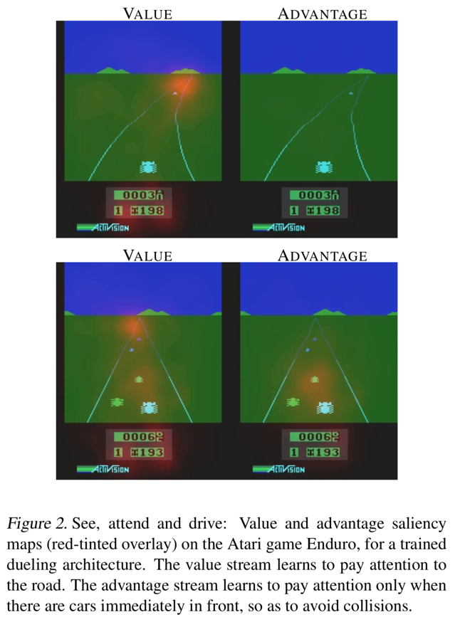
Dueling DQN

• Sometimes:
  • No action is necessary in a state; or
  • It doesn’t matter much which action is done; or
  • One action is better than another in a range of states.
• \(Q(s,a)\) conflates assessing states and assessing values (as would \(U(S)\), then picking action)
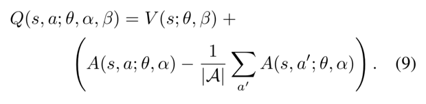
• What if split \(Q(s,a) = V(s) + A(s,a)\)
  • Value of state \(s\) \(V(s)\) is basically \(U(s)\)
  • Advantage of action \(a\) in state \(s\) \(A(s,a)\) is state-dependent action worth

Dueling DQN

• Learn \(V(S)\) and \(A(s,a)\) separately, then recombine to give \(Q(s,a)\):

  

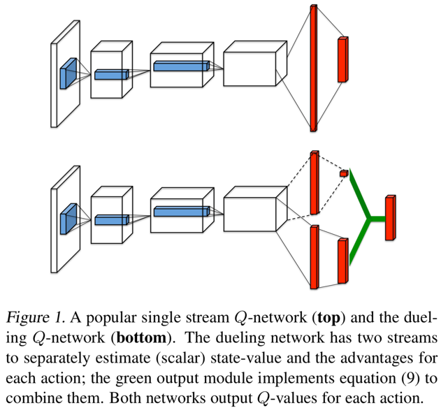
Dueling DQN

Dueling DQN advantage

• Learn values of states when actions don’t matter

• Don’t worry about choosing an action when it doesn’t matter